Welcome to Understanding CRDTs, a series of articles in which we’ll discuss CRDTs from the ground up. We’ll start from the basic concepts, trying to discuss different algorithms and data structures using simple JavaScript implementations, and we’ll gradually work towards a high-performance, JSON CRDT implementation written in Rust.
Chapters (so far):
In the previous article, we implemented a basic Set with support for additions and removals, as well as basic CRDT semantics. Despite working in simple cases, we also highlighted two significant limitations:
- An element cannot be re-added to the Set after being removed
- Although a removal would logically remove an element from the Set, the underlying data structure’s size keeps increasing over time. If we perform many deletions, this could bloat the size of the structure significantly.
In this article, we’ll try to tackle the first problem, discussing different approaches and tradeoffs.
Supporting additions after removals
As we mentioned, our current Set implementation does not allow an element to be restored after being deleted:
const replicaA = new CRDTSet();
replicaA.add("a");
console.log(replicaA.has("a")); // true

const replicaB = new CRDTSet();
replicaB.merge(replicaA);
replicaB.remove("a");
console.log(replicaB.has("a")); // false

replicaA.merge(replicaB);
console.log(replicaA.has("a")); // false

// Add 'a' back
replicaA.add("a");
console.log(replicaA.has("a")); // false! Ouch, it should be true
For some use cases, this is a significant limitation: imaging building a grocery list application. You might add some elements to your “to buy” set, and later remove them after the purchase. This would work for a while, but then you might find yourself needing to buy the same product again. In this case, you would need to add elements to the set again after deleting them.
The reason why we are unable to add an element back after its removal is that our current implementation always prioritizes the removals set. Let’s take the following scenario as an example:
elements = {a, b}
removals = {b}
In this case, our Set will logically contain only element a, as element b is present in the removals set and thus ignored.
Attempt 0: Removing elements
If having b in the removals Set prevents us from restoring it, can’t we simply remove b from removals after re-adding it? For example:
elements = {a, b}
removals = {b}

// Then user calls set.add("b")

elements = {a, b}
removals = {}
Unfortunately, as we’ve seen in the previous chapter, removing elements from our sets becomes problematic once replicas and synchronization enter the picture. In those cases, deleting b from the removals set could cause it to randomly disappear again during synchronization, so we need a better solution.
Attempt 1: Adding timestamps
Let’s take a step back and focus on our expected outcome: our goal is to be able to add an element to the Set after removing it. If we had a way to determine whether our element was added before or after its removal, we could decide whether to ignore it or not. For example, if element b was added after removing element b, then element b should be included, but if element b was added before removing element b, then it should be ignored. In other words, we need some kind of ordering between our Set operations.
An initial approach to achieve ordering is to attach a timestamp to our additions and removals. We are going to do this by converting our elements and removals Sets into Maps:
// Before
elements = {a, b}
removals = {b}

// After
elements = {
  a: "2024-02-24",
  b: "2024-02-23",
}
removals = {
  b: "2024-02-24",
}
In this case, the keys of our map represent the elements, while the values represent the time in which the elements were added or removed.
Note: in the previous example, timestamps are represented as string dates to make them easier to read and understand by humans. This implementation would be quite inefficient in practice, so we are going to use Unix timestamps in the actual code.
The time information will be provided by the add and remove methods:
  add(element) {
    this.elements.set(element, new Date().getTime());
  }

  remove(element) {
    this.removals.set(element, new Date().getTime());
  }
With the time information, we can finally refine our Set logic to support additions after removals:
An element is present in our Set if:
- It’s present in the
elementsand not in theremovals- OR if the timestamp in the
elementsis greater or equal than the timestamp in theremovals
Thanks to the second condition, we are now able to add an element back after its removal. This works because whenever we add an element, we also update its timestamp, and if this timestamp is greater than the current removals timestamp, we consider the element to be present.
A possible implementation for the has method could be:
  has(element) {
    const additionTime = this.elements.get(element);
    if (additionTime === undefined) {
      // Element was never added
      return false;
    }

    const removalTime = this.removals.get(element);
    if (removalTime) {
      // Was the element removed before or after its addition?
      return removalTime <= additionTime;
    }

    // The element was never removed
    return true;
  }
Finally, to make our Set a proper CRDT, we’ll need to update the merge method as well:
  merge(otherSet) {
    for (let [element, additionTime] of otherSet.elements) {
      const existingAdditionTime = this.elements.get(element);
      // Update the local addition time only if the remote addition time is greater
      if (
        existingAdditionTime === undefined ||
        existingAdditionTime < additionTime
      ) {
        this.elements.set(element, additionTime);
      }
    }

    for (let [element, removalTime] of otherSet.removals) {
      const existingRemovalTime = this.removals.get(element);
      // Update the local removal time only if the remote removal time is greater
      if (
        existingRemovalTime === undefined ||
        existingRemovalTime < removalTime
      ) {
        this.removals.set(element, removalTime);
      }
    }
  }
}
We are now ready to test our Set again (the full code is available here):
  const replicaA = new CRDTSet();
  replicaA.add("a");
  console.log(replicaA.has("a")); // true

  // Wait for some time between operation.
  // This way, the new Date.getTime() call can't return the same value
  await waitFor(10);

  const replicaB = new CRDTSet();
  replicaB.merge(replicaA);
  replicaB.remove("a");
  console.log(replicaB.has("a")); // false

  await waitFor(10);

  replicaA.merge(replicaB);
  console.log(replicaA.has("a")); // false

  await waitFor(10);

  replicaA.add("a");
  console.log(replicaA.has("a")); // true! Yay, 'a' is back!
Yay, our Set can now handle additions after removals! Is this ready for production? Well, not exactly. Our current implementation suffers from a subtle, but very problematic edge case, which we’ll discuss in the next section.
Physical time and distributed systems
In the implementation we just discussed, timestamps play an important role: they allow us to tell which operation comes first. In other words, we are relying on timestamps to determine the ordering of operations, which in turn determines which elements are present in the set and which are not. Unfortunately, this approach can break down in subtle ways when dealing with distributed systems.
Most of our devices, including laptops and mobile phones, rely on a hardware device to keep track of time: the clock. These clocks are usually based on quartz oscillators and are not very precise, so every device has its own notion of time. For example, this is a picture of my car’s clock:

Every few weeks, I might need to adjust the time, as it might have drifted by one or two minutes. Some of you might be wondering: why isn’t this time drift happening on our phones and laptops? Well… it is! The reason we don’t notice is a protocol known as NTP (Network Time Protocol), which allows internet-connected devices to periodically sync their time with NTP servers, down to a <100ms precision. Unfortunately, my car is quite old and doesn’t have any kind of internet connectivity, so NTP is not an option there. Until I keep my car, I’ll need to keep the time up to date manually (though as you can see from the year, I’m not particularly good at it :D ).
As long as the NTP protocol works, our devices will have a reasonably precise clock, so why shouldn’t we rely on timestamps for the operation ordering?
In software systems, data integrity is usually one of the top concerns. For example, let’s take two hypothetical bugs:
- A bug causing application instances to crash
- A bug silently corrupting data in our database
Which one sounds scarier?
As a result, when designing a data structure like our CRDT Set, we should always think about the worst-case scenarios: what happens if the time in our local machine goes off? Let’s see an example, starting from this Set state:
elements = {
  a: "2024-02-24",
  b: "2024-02-23",
}
removals = {}
Let’s say for some reason, our local time is completely off and we decide to remove element b. As we discussed before, this causes a new entry to be added to the removals map:
elements = {
  a: "2024-02-24",
  b: "2024-02-23",
}
removals = {
  b: "2099-02-24",  // <- year is set to 2099
}
From the user perspective, this works correctly: the element b is removed (because 2099 > 2024).
After a while, the CRDT Set is replicated to another replica, which might decide to add element b again. As a result, we update the timestamp of entry b in the elements map:
elements = {
  a: "2024-02-24",
  b: "2024-02-24", // <- updated, but still less than 2099!
}
removals = {
  b: "2099-02-24",
}
But this time, the b element does not come back… In fact, it will not come back for the next 75 years! By relying on physical timestamps to determine the order of operations, we might cause silent data loss or corruption in the case of out-of-time clocks. We can do better than that.
Aside: How likely is this out-of-time scenario to happen?
Despite being a rare occurrence, these are some scenarios in which a device’s time could experience some edge-case behaviors:
- Firewalls could be misconfigured and temporarily block NTP synchronization, making the local clock slowly drift over time.
- When the drift between the local clock and the NTP server clock is too large, the NTP protocol might decide to reset the local clock. From the perspective of local applications, the clock would have jumped forward or backward in time.
- Users could even misconfigure their local time on purpose, for example, trying to elude “trial periods” of certain proprietary software.
If you want to know more about this topic, I highly recommend reading the “Unreliable Clocks” chapter from Designing Data-Intensive Applications by Martin Kleppmann, one of the best software engineering books ever written.
So if physical timestamps are not a good option for this use case, what should we use? A better mechanism to determine the order of operations in distributed systems is Version Vectors, which we are going to cover in the next section.
Attempt 2: Version Vectors
Version Vectors are a mechanism for tracking changes to data in a distributed system. Most importantly, they can do so without relying on physical time.
To introduce Version Vectors, let’s imagine a distributed scenario in which two replicas exist. We’ll call them Alice and Bob:
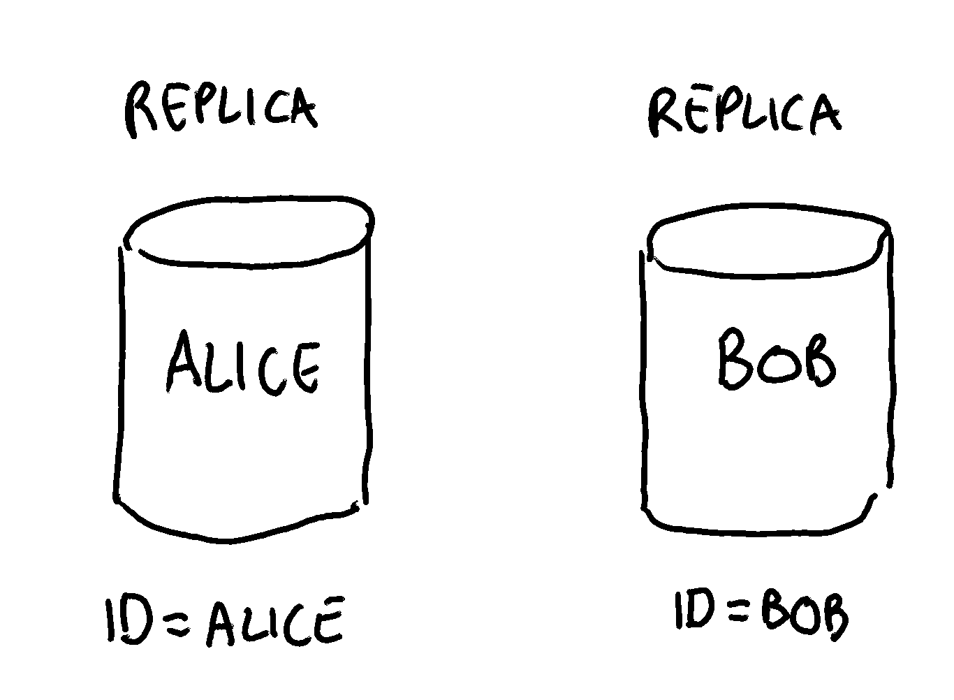
When using Version Vectors, each replica has to have a unique ID, which we’ll call replica ID. For simplicity, Alice will have ID = alice and Bob will have ID = bob.
Version Vectors can be thought of as maps, in which the keys are the replica IDs and the values are the number of changes to the data by the given replica. For example, when Alice adds a new element, the corresponding Version Vector will be:
{alice: 1}
which can be read as “Alice has made one edit to the data so far”. If Alice performs another update, the Version Vector will become:
{alice: 2}
And if this value is then modified by Bob, the Version Vector will become:
{alice: 2, bob: 1}
which can be read as “Alice has made 2 edits to the data, while Bob made one edit”.
When executing an operation (either add or remove ), our CRDT Set will attach a Version Vector to the value, in the same way as we did with the timestamps:
elements = {
  a: {alice: 1},
  b: {alice: 2},
}
removals = {
  b: {alice: 2, bob: 1}
}
All good so far, but we still haven’t discussed how Version Vectors can help us. To answer that question, let’s take a step back: our goal is to determine whether a removal occurred before or after the corresponding addition, as that will determine whether the element is present in the set or not. In other words, we need a way to determine an ordering between the additions and removals of the same element. Version Vectors serve exactly that purpose, let’s see how:
Every time a replica executes an operation on a given element, it increments the corresponding counter in the Version Vector:
VV = {alice: 1}

// After an operation by Alice
VV = {alice: 2}
Because we know that replica IDs are unique (more on this below), we can derive a partial ordering by comparing two version vectors. For example, given these two Version Vectors:
{alice: 1}
{alice: 2}
we know that {alice: 2} must have come after {alice: 1} (because the replica IDs are unique and each operation causes an increment in the current replica counter). For example, let’s consider the following scenario:
elements = {
  a: {alice: 1},
}
removals = {
  a: {alice: 2}
}
In this case, because {alice: 2} comes after {alice: 1}, we know that element a was removed. On the other hand, the following scenario displays a Set in which the element a is present:
elements = {
  a: {alice: 3}, // <- 3 is greater than 2, so 'a' is present
}
removals = {
  a: {alice: 2}
}
When multiple replicas modify the same data, each replica increments its own counter. For example:
VV = {alice: 1}

// After Bob modifies the data
VV = {alice: 1, bob: 1}
By comparing these two version vectors, we know that {alice: 1, bob: 1} comes after {alice: 1}, because the former is a superset of the latter. In other words, a version vector A is greater than a version vector B if all counters of A are greater or equal to the corresponding counters on B.
So in the following scenario, we know that a is not present in the Set:
elements = {
  a: {alice: 1},
}
removals = {
  a: {alice: 1, bob: 1} // <- This VV is greater than {alice: 1}
}
The trickiest scenario happens when two replicas modify the same data concurrently:
VV = {alice: 1}

// Alice modifies the value
VV = {alice: 2}
// At the same time, Bob modifies the value
VV = {alice: 1, bob: 1}
Does {alice: 2} come before or after {alice: 1, bob: 1}? Neither of the two! The two version vectors are concurrent. In other words, we can’t tell which update came first by just looking at their version vectors. What should we do in this case? Let’s discuss an example to illustrate a possible approach.
Let’s assume both Alice and Bob start from the following state:
elements = {
  a: {alice: 1},
}
removals = {}
From the rules we discussed before, we know that this Set contains element a .
Then, each replica updates its set concurrently. In particular, Alice removes and then adds a again:
elements = {
  a: {alice: 3},
}
removals = {
  a: {alice: 2}
}
While Bob only removes a, without adding it back:
elements = {
  a: {alice: 1},
}
removals = {
  a: {alice: 1, bob: 1}
}
When the two replicas synchronize, a conflict occurs: should a be present or not? Should the actions of Alice take precedence over the ones from Bob, or vice versa? It depends on the application, as different use cases require different approaches.
A safe approach we could use is prioritizing additions over removals when a conflict occurs, a policy known as Add Wins. According to this logic, if some replica deletes an element while another replica adds it, then the addition should “win”. This policy is the safest as it minimizes the risk of unwanted data loss. For example, it would be easy for Bob to remove element a again if he’s really convinced about his choice, with minimal UX impact. But if we didn’t adopt the Add-Win policy, Alice might have element a silently disappear after the synchronization, which could lead to a bad UX.
Note: Different approaches to conflict resolution are possible, the most suitable of which depends on the specific use case. For example, some applications might require to “merge” elements when a conflict occurs, rather than having one override the other. Others might prefer the removal operation to take precedence.
If we opt for the Add-Wins policy in our CRDT Set, Alice’s addition will win over Bob’s removal. The only thing left to figure out is what the Version Vector will be.
When a conflict occurs, we are going to merge the two Version Vectors. A merge consists of creating a Version Vector whose counters are the maximum value across all conflicting vectors’ counters. For example, merging {alice: 2} with {alice: 1, bob: 1} will result in {alice: 2, bob: 1}. By applying this logic to our previous example, we’ll end up with the following state:
elements = {
  a: {alice: 3, bob: 1}, // <- merged vector
}
removals = {
  a: {alice: 2} // The value of the removals version vector doesn't really matter, as long as it's smaller than the addition version vector
}
The resulting set will contain element a , because the resulting vector ({alice: 3, bob: 1} ) is greater than the vector in removals.
An important side-effect of the merge, which might not be obvious at first, is that the resulting version vector now “encodes” the fact that it came after both concurrent updates. In other words, we can tell for sure that this addition comes after both Alice’s addition and Bob’s removal. This allows us to accurately track the way our data evolves when multiple replicas update it.
We now have all the necessary ingredients to implement our Version Vector CRDT Set in JS. Because the implementation is quite long, I’ve decided to not include it in the article, but you can find it on the GitHub repo here.
All right! We now have implemented a CRDT Set that supports additions, removals, and concurrent updates without relying on physical clocks, making it more robust for use in distributed systems.
Remarks on Replica IDs
An important discussion we should have is related to Replica IDs. Version Vectors (as well as other approaches we’ll discuss in the upcoming chapters) rely on the fact that every replica has a unique ID. Without the uniqueness guarantee, we couldn’t infer an ordering between two Version Vectors. For example, if two replicas had Alice as replica ID, we couldn’t tell for sure if the version vector {alice: 2} comes after {alice: 1}. We can infer an ordering only when we can safely assume that a replica counter will only be incremented by a single replica (based on the ReplicaID).
You will find this ID uniqueness requirement in most CRDT implementations. In fact, many CRDTs explicitly mention that it’s up to you to guarantee unique replica IDs, otherwise you might face data corruption (eg. here).
This requirement is made more complex by the fact that CRDTs are typically used in distributed P2P scenarios. In those cases, we can’t rely on a central authority to assign IDs that are guaranteed to be globally unique. The most popular solution in those cases is to generate a random replica ID large enough to be statistically unlikely to conflict with another replica ID. The downside of large replica IDs is that they can take up quite a bit of storage within our CRDT, depending on the implementation. So in these cases, we need to balance our accepted risk of data corruption with our efficiency requirements or introduce a global “coordination” entity to assign unique IDs.
Remarks on Version Vectors storage
Version Vectors are a powerful tool in our distributed systems toolbox. Their main downside is that they can take quite a bit of storage in our data structure, and in certain scenarios, a lot of storage.
The ideal scenario for Version Vectors is when any given data entry is only ever modified by a single replica:
VV = {alice: 1}
VV = {alice: 2}
VV = {alice: 3}
As you can see, because our data is only modified by Alice, our Version Vector’s size doesn’t grow.
If at some point another replica decides to modify the data, our Version Vector’s size grows by one:
VV = {alice: 3, bob: 1}
Therefore, the worst-case scenario happens when a data entry is modified by a different replica every time:
VV = {alice: 1}
VV = {alice: 1, bob: 1}
VV = {alice: 1, bob: 1, carl: 1}
VV = {alice: 1, bob: 1, carl: 1, david: 1}
That adds up quickly!
The problem is that we can fall into this worst-case scenario quite easily if we are not careful. For example, given that replica IDs have to be unique, we could decide to solve the problem by generating a random ID every time our CRDT is initialized. At this point, every time we modify the same entry, the Version Vector size will grow by one. Given that our CRDT is likely to be initialized at least once every time the user starts our application, modifying the same entries will cause the Version Vector size to grow fast!
For some use cases, this might not be a significant problem, for example in scenarios in which the creation of new objects is more common than edits or when Replica IDs can be reused among different sessions. There is also a more efficient version of Version Vectors called Dotted Version Vectors, which in some cases can bring significant space savings. We’ll hopefully cover it in a future chapter of the series, so stay tuned :)
Conclusions
That was quite a ride! We finally have a working CRDT Set implementation, but there is still a lot to discuss:
- Our CRDT Set only keeps growing over time, even after we remove elements. Can we implement deletes more efficiently?
- When we synchronize the replicas of our CRDT, we currently need to send the entire state to each other, which could become prohibitive expensive after a certain size. Can we implement a more efficient synchronization in which only the “new” data is sent over the wire?
- What about other data structures like Lists and Maps?
These will be the topics of the next chapters, so stay tuned!
PS: All the code is available in this repository: https://github.com/federico-terzi/crdt-experiments